1 · Tolerance-aware vs tolerance-unaware
1.1 · Tolerance-aware vs tolerance-unaware Click to expand
Setup. Tolerance-aware optimisation evaluates E[M], i.e the expected merit over the fabricated lenses in closed form per ray using the propagation of uncertainty (POU) method. The tolerance-unaware line is the baseline (optimised for merit M at the nominal design, no perturbations). Both 10 000 iterations, three seeds per na_weight.
2 · Tolerance-tightening curriculum
2.1 · Tolerance-aware + curriculum vs tolerance-unaware Click to expand
Setup. Five stages per na_weight, 2000 iterations each, each stage warmstarted from the previous one. The perturbation σ is annealed 8× → 4.76× → 2.83× → 1.68× → 1× of the precision spec, so the final stage optimizes at the target tolerance.
Result. The curriculum frontier has a much narrower tolerance spread than the tolerance-unaware baseline at matched throughput.
3 · Vignetting term
3.1 · With and without the vignetting term, vs nominal Click to expand
Objective. The merit of a single lens is unchanged throughout — spot error against throughput averaged over the five field angles:
The tolerance-aware objective is the expectation of that merit over the perturbation distribution, which POU evaluates in closed form. That is the κ = 0 series:
A field angle with no surviving rays contributes zero to both averages inside M, so E[M] can be lowered by driving the outer field to zero throughput.
Evaluating E[M] yields the expected per-angle throughputs E[Ta] as an intermediate. The κ = 1 series adds a penalty on their spread:
κ = 0 recovers the previous objective exactly.
Both series: 150 000 iterations, learning rate 1e-3, 1024 rays per field angle, precision tolerance grade, identical in every setting but κ.
The tolerance-unaware baseline in the plot was run at 10 000 iterations and 128 rays per field angle, so it is not matched in compute to the two POU series.
4 · Volume renders
4.1 · Absolute scale Click to expand
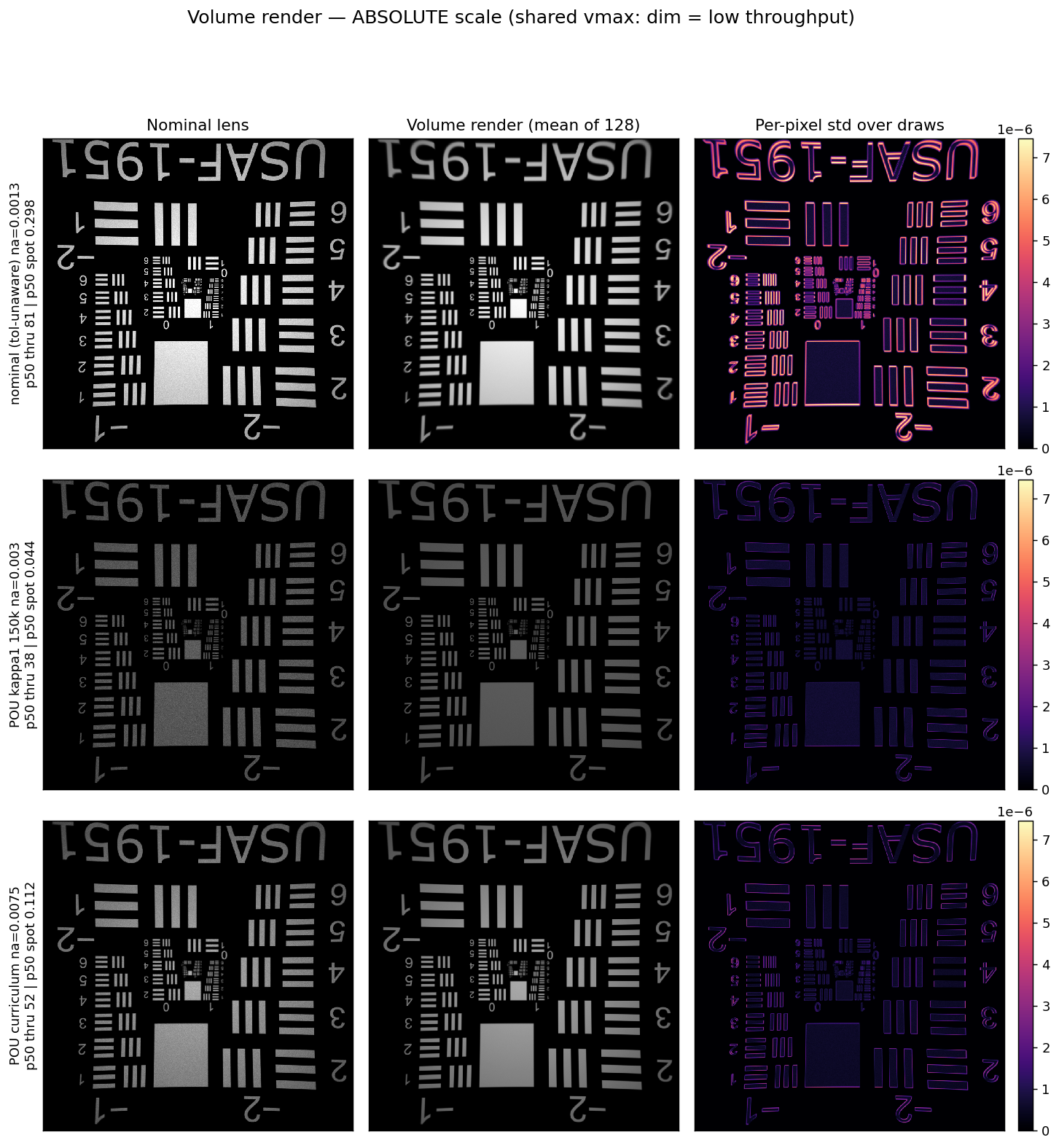
Setup. Volume render: expected render over the sampled lenses: here we do 128 lens draws from the precision-grade tolerance model, each rendered separately (1024×1024, 800 spp), then averaged.
| design | p50 throughput | p05 spot | p50 spot | p95 spot | mean spot |
|---|---|---|---|---|---|
| nominal (tolerance-unaware) na=0.0013 | 81.1 | 0.040 | 0.298 | 2.139 | 0.605 |
| POU κ=1 150k na=0.003 | 38.3 | 0.034 | 0.044 | 0.103 | 0.055 |
| POU curriculum na=0.0075 | 52.2 | 0.089 | 0.112 | 0.213 | 0.128 |
All panels share one intensity scale, so brightness is cross-comparable.
Draw statistics are over these 128 draws
4.2 · Exposure-matched Click to expand
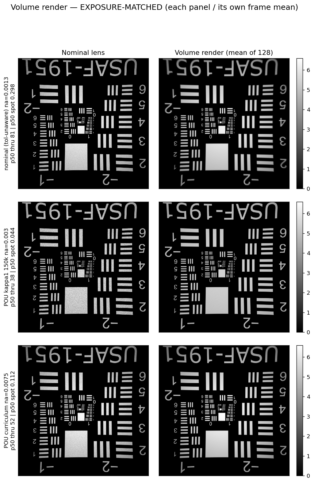
Setup. Each panel is divided by its own frame mean, then all share one scale. To better see the "blur" comparison, equivalent to giving each camera its own exposure time.
4.3 · Interactive comparison Click to expand
Hover a tab or press 1–9 to swap the large image; move the cursor over it to magnify the same spot in every design at once. Tabs 1–3 are the exposure-matched volume renders, 4–6 the same designs' nominal lenses, 7–9 the volume renders on the absolute scale.